4. Change detection aggregation#

The overall scheme of the L2b processing is reported in figure below.

The key step is fusion of L2a estimates at map level. These steps are described in detail in the following subsections.

The step is mandatory.

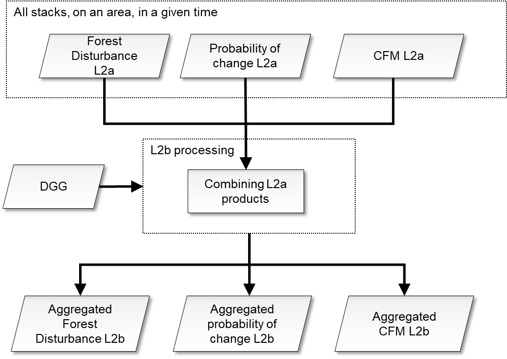
Complete flow-chart of the L2b processing.

Fig. 14 — Complete flow-chart of the L2b processing.

4.1 Fusion of L2a products on a Tile within a fixed timespan#

4.1.1 Overview and rationale#

The disturbance maps allow the combination of different acquisitions in a simple and efficient pixelwise way. L2a products falling onto the same L2b tile within a global cycle are retrieved through geospatial query of information (tile IDs and time tags) in the Main Product Header of the product.

From the disturbance map combined, the extraction of the combined CFM is obtained by a simple logical and operator.

L2a FD fusion.

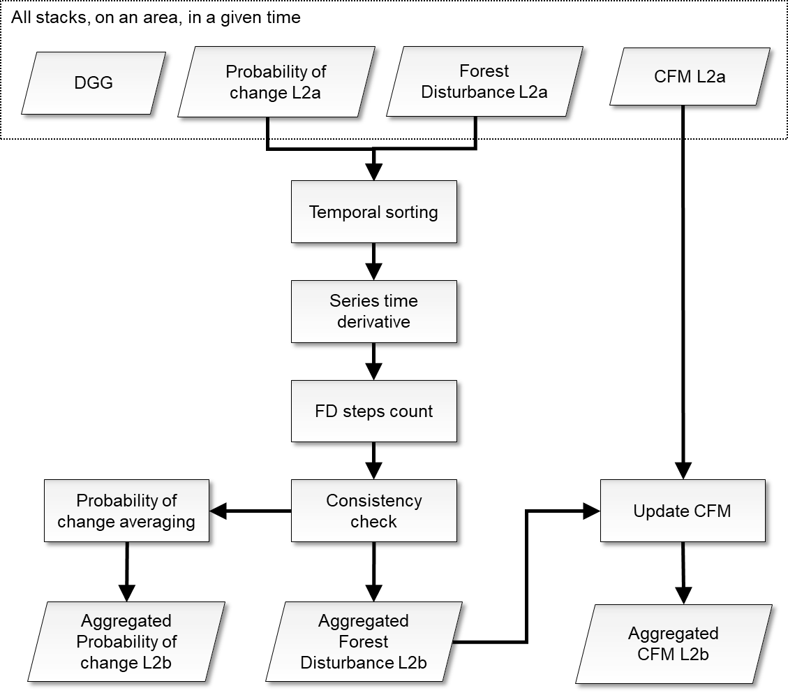
Fig. 15 — L2a FD fusion.

4.1.2 Inputs#

Symbol	Name	Origin	Size	Variability	Default	Description
\({{FD}_{map}}^{t^i}\)	Forest Disturbance	FD L2a products in a DGG tile in a global cycle (`FD_PFD`)	\(\left[ N_{lat}\times{}N_{lon} \right]^{t^i}\)	-	-	Forest Disturbance map
\({CFM}^{t^i}\)	CFM	FD L2a products in a DGG tile in a global cycle (`FD_PFD`)	\(\left[ N_{lat}\times{}N_{lon} \right]^{t^i}\)	-	-	CFM
\({P_c}^{t^i}\)	Probability of change	FD L2a products in a DGG tile in a global cycle (`FD_PFD`)	\(\left[ N_{lat}\times{}N_{lon} \right]^{t^i}\)	-	-	Probability of change map
DGG	DGG	Internal lookup table	-	-	-	DGG tile
BBi	Footprint	L2a main product header (`FD_PFD`)	lat-lon vertices (4 couples)	-	-	The extent of the L2a input data in geographical coordinates
mDGG	`minimumL2aCoverage`	`AUX_PP2_` FD (`AUX_FMT`)	float value [scalar]	0.0-100.0	10.0	The minimum [%] tile coverage that triggers the computations

4.1.3 Outputs#

Symbol	Name	Destination	Size	Variability	Default	Description
\({{FD}_{map}}^{aggregated}\)	Forest Disturbance	FD L2 b product (`FD_PFD`)	\(\left[ N_{lat,L2b}\times{}N_{lon,L2b} \right]\)	-	-	Forest Disturbance map aggregated
\({CFM}^{aggregated}\)	CFM	FD L2 b product (`FD_PFD`)	\(\left[ N_{lat,L2b}\times{}N_{lon,L2b} \right]\)	-	-	CFM aggregated
\({P_c}^{aggregated}\)	Probability of change	FD L2 b product (`FD_PFD`)	\(\left[ N_{lat,L2b}\times{}N_{lon,L2b} \right]\)	-	-	Probability of change map aggregated
HM	heat map	FD L2b product (`FD_PFD`)	\(2\left[ N_{lat,L2b}\times{}N_{lon,L2b} \right]\)	0-	-	heat map (couple of integer values per pixel)

4.1.4 Algorithm mathematical background#

As a first step, the minimum required coverage over L2b DGG tile j is checked to proceed with computations:

(1)#\[TR=\ (100*\frac{A(\left. \bigcup_i^{}{{BB}^i} \right\vert_{DGG}\cap\left. {TT}^j \right\vert_{DGG})}{A(\left. {TT}^j \right\vert_{DGG})}>mDGG) \tag{4.1}\]

where BBi are the L2a bounding boxes, TTj is the footprint of the current L2b DGG tile and A operator computes the area of the corresponding polygon.

The aggregation at pixel map level of the various L2a disturbance maps is done by examining the consistency of the time series of detections. First, the series of detection is temporally sorted, both ascending and descending orbits:

(2)#\[{{FD}_{series}}^{sorted}(t)=\left\{ {{FD}_{map}}^{t^1},...,{{FD}_{map}}^{t^i}\ \right\} \tag{4.2}\]

\(\left\{ t^1<...<t^i\ \right\}\) being the different times at which each product is acquired in a global cycle. Then the derivative of the sorted time series is computed with respect to time and thresholded

(3)#\[{{FD}_{series}}^{steps}=\left\vert \frac{d\left[ {{FD}_{series}}^{sorted}(t) \right]}{dt} \right\vert>0 \tag{4.3}\]

Finally, the number of transitions in the derivative vector is counted

(4)#\[{{FD}_{steps}}^{count}=\sum_i^{}{{{FD}_{series}}^{steps}(i)} \tag{4.4}\]

If the sum is odd, detection is assumed, and the resulting probability of change is the average of the different probabilities pixel-wise for detection only. Otherwise, the resulting probability of change and FD map is set to zero. If the sum is zero, detection is assumed only if all the acquisitions show detection. The rationale is that change is assumed only if all the acquisitions detecting it are simultaneously consistent. The situation is depicted in Fig. 16 for the example of three acquisitions and the corresponding truth table is reported in Tab.1.

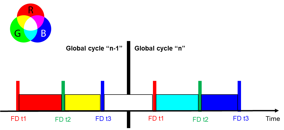
Time of validity for each acquisition among two global cycles, with overlaps shown in RGB colours. The FD relative to various acquisition times within the global cycle are reported. See also Tab.1.

Fig. 16 — Time of validity for each acquisition among two global cycles, with overlaps shown in RGB colours. The FD relative to various acquisition times within the global cycle are reported. See also Tab.1.

Table 1 — Truth table for the example of three FDs. The color coding for FD t1/3 is the same of Fig.16, where black is the absence of validity.

FD t1	FD t2	FD t3	FD steps count	FD map aggregated	HM: contributing	HM: agreeing
0	0	0	0	0	3	3
0	0	1	1	1	3	1
0	1	0	2	0	3	2
1	0	0	1	1	3	1
1	1	0	1	1	3	2
1	0	1	2	0	3	1
0	1	1	1	1	3	2
1	1	1	0	1	3	3

A heat map HM is also stored representing at pixel level:

the total number of acquisitions contributing to the decision, as reported in Tab.1 – column 6
the number of acquisitions agreeing to the decision, as reported in Tab.1 – column 7

From the disturbance map combined, the extraction of the forest mask is obtained by a simple update to the initial forest mask.

(5)#\[{CFM}^{aggregated}=\left\{ 1-{{FD}_{map}}^{aggregated} \right\}\land\left\{ \cup_{t^i}{CFM}^{t^i} \right\} \tag{4.5}\]

\(\left\{ t^1<...<t^i\ \right\}\) being the different times at which each product is acquired in a global cycle, where \(\cup\) is the union operator.